Every metric in fiscal returns four columns — the raw
ratio plus winsorized (_w), standardized (_z),
and percentile-rank (_p) versions. This article explains
what those transformations do, the range codes that control
them, and the distribution-aware machinery behind
find_best_normalization().
Why bother? Nonprofit financial ratios are notoriously badly behaved: heavy right tails (a few enormous organizations), structural zeros (a nonprofit with no debt), hard bounds (a program-expense ratio can’t exceed 1), and the occasional data-entry outlier. Feeding raw ratios into a z-score or a composite index lets those pathologies dominate. Normalization tames them so that comparisons and indices reflect position, not scale artifacts.
Three steps behind every metric column
For a raw ratio, the package:
-
Winsorizes — clips extreme tails to a percentile
bound (
_w). -
Normalizes — applies a distribution-aware
transformation (chosen by
find_best_normalization(), below) and robustly centers and scales the result into a z-score (_z). -
Ranks — expresses each raw value as a percentile,
1–100 (
_p).
apply_transformations() is the engine that does all
three at once. It is what each get_*() function calls
internally:
set.seed(1)
ratio <- c(rlnorm(500, 0, 0.6), 40, 55)   # a right-skewed ratio with two outliers

tf <- apply_transformations(ratio, winsorize = 0.98, range = "zp")
str(tf)
#> List of 4
#>  $ raw       : num [1:502] 0.687 1.116 0.606 2.604 1.219 ...
#>  $ winsorized: num [1:502] 0.687 1.116 0.606 2.604 1.219 ...
#>  $ z         : num [1:502] -0.57 0.263 -0.748 2.133 0.436 ...
#>   ..- attr(*, "transform_type")= chr "asinh"
#>   ..- attr(*, "transform_label")= chr "Asinh transformation."
#>   ..- attr(*, "transform_note")= chr "Applied asinh(x / s) with s = 0.97012."
#>   ..- attr(*, "guess_reason")= chr "Variable is nonnegative and not primarily bounded in [0,1]."
#>   ..- attr(*, "center")= num 0.881
#>   ..- attr(*, "scale")= num 0.39
#>   ..- attr(*, "range")= chr "zp"
#>   ..- attr(*, "winsorize")= num 0.98
#>   ..- attr(*, "offset")= num 0.001
#>   ..- attr(*, "fit_object")=List of 24
#>   .. ..$ range               : chr "zp"
#>   .. ..$ support             :List of 6
#>   .. .. ..$ code       : chr "zp"
#>   .. .. ..$ lo         : num 0
#>   .. .. ..$ hi         : num Inf
#>   .. .. ..$ sentinel_lo: num -0.001
#>   .. .. ..$ sentinel_hi: num NA
#>   .. .. ..$ offset     : num 0.001
#>   .. ..$ winsorize           : num 0.98
#>   .. ..$ offset              : num 0.001
#>   .. ..$ standardize         : logi TRUE
#>   .. ..$ robust              : logi TRUE
#>   .. ..$ transform_type      : chr "asinh"
#>   .. ..$ guess_reason        : chr "Variable is nonnegative and not primarily bounded in [0,1]."
#>   .. ..$ zero_tol            : num 1e-08
#>   .. ..$ one_tol             : num 1e-08
#>   .. ..$ boundary_mass_cutoff: num 0.1
#>   .. ..$ hurdle_trans        : chr "rank"
#>   .. ..$ hurdle_range        : num [1:2] 1 100
#>   .. ..$ n_clean             : int 491
#>   .. ..$ raw_skewness        : num 1.21
#>   .. ..$ raw_kurtosis        : num 1.36
#>   .. ..$ transform_label     : chr "Asinh transformation."
#>   .. ..$ transform_note      : chr "Applied asinh(x / s) with s = 0.97012."
#>   .. ..$ params              :List of 1
#>   .. .. ..$ scale_const: num 0.97
#>   .. ..$ standardization     : chr "robust"
#>   .. ..$ center              : num 0.881
#>   .. ..$ scale               : num 0.39
#>   .. ..$ fit_skewness        : num 0.48
#>   .. ..$ fit_kurtosis        : num -0.332
#>   .. ..- attr(*, "class")= chr "normalize_x_fit"
#>  $ pctile    : int [1:502] 25 57 18 94 61 19 68 77 72 38 ...
summary(data.frame(raw = tf$raw, w = tf$winsorized, z = tf$z, p = tf$pctile))
#>       raw                w                z                  p
#>  Min.   : 0.1645   Min.   :0.1645   Min.   :-1.82645   Min.   :  1.0
#>  1st Qu.: 0.6889   1st Qu.:0.6889   1st Qu.:-0.56492   1st Qu.: 25.0
#>  Median : 0.9790   Median :0.9790   Median : 0.01661   Median : 50.0
#>  Mean   : 1.4062   Mean   :1.2124   Mean   : 0.23062   Mean   : 50.3
#>  3rd Qu.: 1.5102   3rd Qu.:1.5102   3rd Qu.: 0.88289   3rd Qu.: 75.0
#>  Max.   :55.0000   Max.   :3.7557   Max.   : 3.02864   Max.   :100.0
Notice the two outliers (40, 55) are pulled back in the winsorized column, which keeps them from dominating the z-score. The percentile rank depends only on ordering, so extreme values cannot distort it either way.
The range codes
Winsorization and transformation both need to know a variable’s
theoretical support — a program-expense ratio lives in
[0, 1]; a growth rate can be negative; a dollar amount is
non-negative and unbounded above. The range argument
encodes this:
| Code | Support | Typical metric |
|---|---|---|
"np" |
negative → positive | growth rates, margins |
"zp" |
zero → positive | dollar amounts, days of cash |
"zo" |
zero → one | expense/revenue share ratios |
"nz" |
negative → zero | (rare) strictly non-positive measures |
"lo;hi" |
a custom pair | e.g. "0;10" for a bounded index |
The support determines where winsorization clips and
which transformation is appropriate. winsorize_x()
exposes the winsorization step directly:
w <- winsorize_x(ratio, range = "zp", winsorize = 0.98)

c(bottom = w$bottom, top = w$top)
#>    bottom       top
#> -0.001000  3.755658
sum(w$is_sentinel)     # observations pushed to a bound
#> [1] 11
find_best_normalization(): distribution-aware
transformation
Standardizing a badly skewed variable produces a badly skewed
z-score. For multivariate work — correlations, factor analysis, the
fiscal-health index — we want each indicator to be approximately
normal first. find_best_normalization() does this by
choosing, per variable, one of three transformations (a fourth,
hurdle, is available on request) based on the shape of its
stable interior (the non-sentinel, non-missing values
left after winsorization).
The procedure is always the same:
- Winsorize and set aside sentinel (boundary) observations so pile-up at the bounds can’t distort the fit.
- Diagnose the stable interior — its support, boundary mass, and zero inflation.
-
Select a transformation from those diagnostics (or
accept an explicit
vtype). - Fit the transformation’s parameters and a robust center/scale (median / MAD, falling back to mean / SD when the MAD is zero because more than half of the transformed values are tied).
- Report before-and-after skewness and kurtosis so you can see whether the transformation actually helped.
Separating fit from apply means the same fitted
model can score a later panel year on an identical scale — see
apply_normalization() at the end.
How the transformation is chosen
guess_normalize_type() implements the decision rule.
Writing p0 for the share of values at zero, p1
for the share at one, and using a boundary_mass_cutoff of
0.10:
is the variable effectively in [0, 1]?  (range "zo", or >98% of values in [0,1])
├── yes
│    ├── p0 > 0.10  ........................  rank_normal  (zero-inflated)
│    ├── p1 > 0.10  ........................  rank_normal  (piled up at the top)
│    └── otherwise  ........................  logit        (well-spread proportion)
└── no
     ├── non-negative? (range "zp", or min >= 0)  ....  asinh   (heavy right tail)
     └── mixed / irregular support  ................  rank_normal
hurdle never comes out of this rule; it is used only
when you ask for it with vtype = "hurdle".
The four transformations, and the distribution pathology each one targets:
asinh — heavy-tailed magnitudes
Pathology. Non-negative amounts with a long right
tail: a handful of huge organizations stretch the scale (dollar figures,
days of cash). Transform. The inverse hyperbolic sine
asinh(x / s), scaled by s, the median absolute
non-zero value of the stable interior. It behaves like the identity near
zero and like a log in the tails, is defined at zero, and
accommodates negatives.
set.seed(1)
x_asinh <- rlnorm(2000, meanlog = 10, sdlog = 1.3)   # e.g. total-asset dollars

fit <- find_best_normalization(x_asinh, range = "zp", verbose = FALSE)
c(type = fit$transform_type,
  raw_skew = round(fit$raw_skewness, 2), fit_skew = round(fit$fit_skewness, 2),
  raw_kurt = round(fit$raw_kurtosis, 2), fit_kurt = round(fit$fit_kurtosis, 2))
#>     type raw_skew fit_skew raw_kurt fit_kurt
#>  "asinh"   "2.56"   "0.81"   "7.44"  "-0.19"

plot_normalize_x(x_asinh, range = "zp")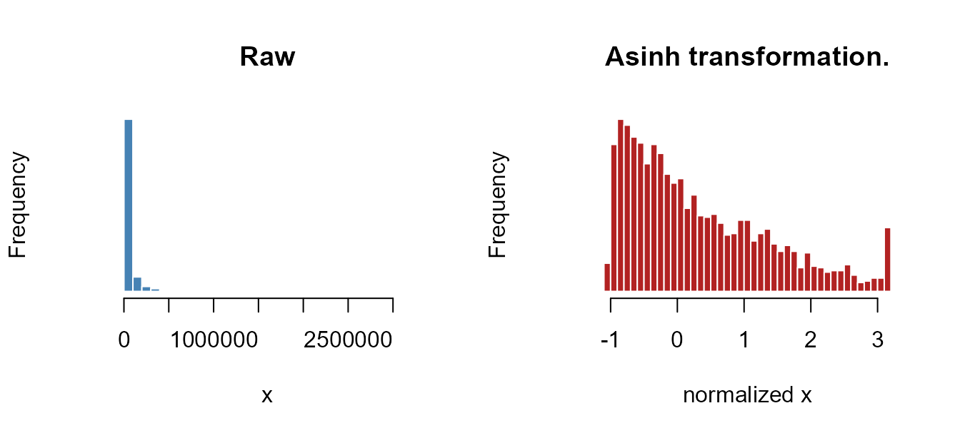
A raw skewness above 2 drops sharply, and the extreme kurtosis is tamed.
logit — well-behaved proportions
Pathology. A ratio bounded in [0, 1]
with mass spread through the middle and little pile-up at the ends (many
expense- and revenue-share ratios). Transform. Rescale
to [0, 1] relative to the theoretical support, then apply
qlogis() (the log-odds), which stretches the bounded scale
onto the whole real line. Before the log-odds, values are clamped to the
(1 - winsorize) / 2 and
1 - (1 - winsorize) / 2 quantiles of the strictly interior
values (those not exactly 0 or 1). An exact 0 or 1 is therefore scored
at the edge of the interior distribution instead of at an extreme
log-odds that would dominate the center, the scale, and any
correlation.
set.seed(2)
x_logit <- rbeta(2000, 2, 8)   # a right-skewed share ratio

fit <- find_best_normalization(x_logit, range = "zo", verbose = FALSE)
c(type = fit$transform_type,
  raw_skew = round(fit$raw_skewness, 2), fit_skew = round(fit$fit_skewness, 2))
#>     type raw_skew fit_skew
#>  "logit"   "0.81"  "-0.39"

plot_normalize_x(x_logit, range = "zo")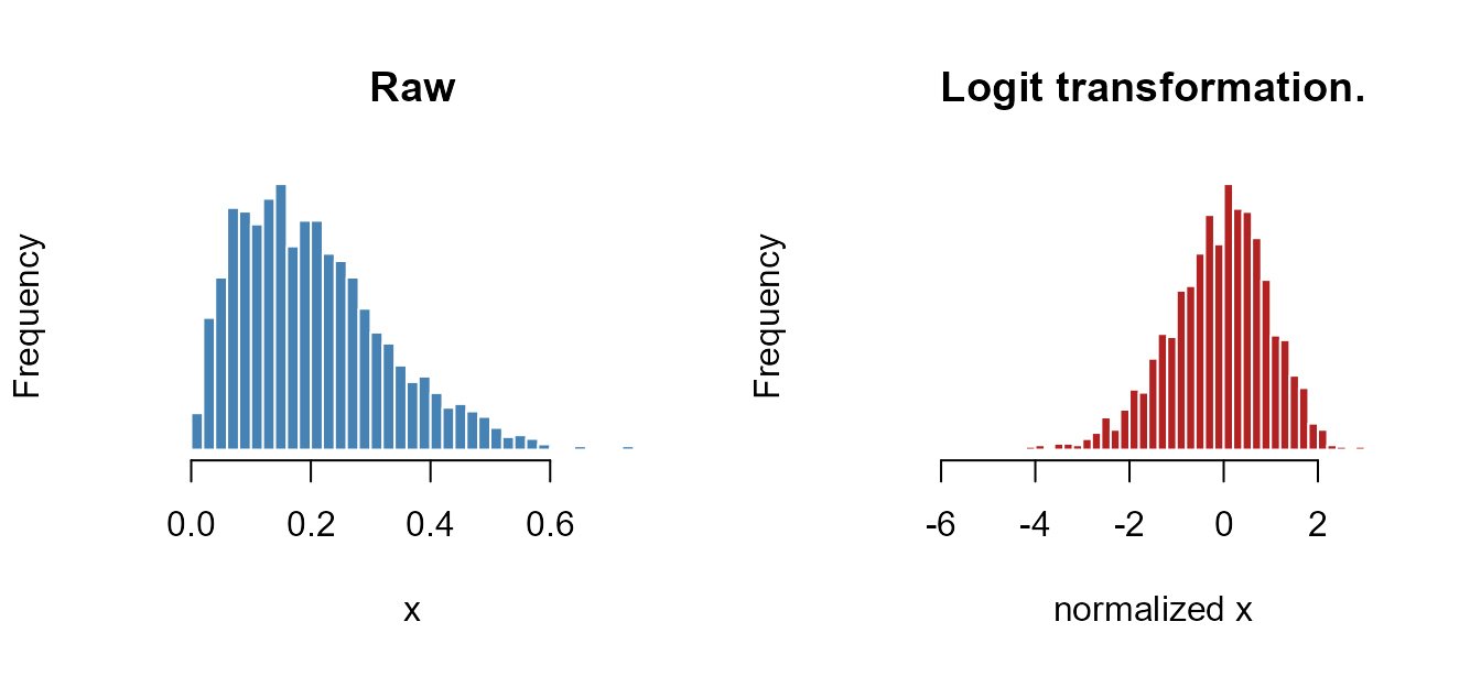
hurdle — structural zeros (on request)
Pathology. A [0, 1] variable with a
spike of exact zeros — organizations that simply don’t do the
thing (no fundraising, no grants, no debt) — mixed with a continuous
positive part. You may want the zeros treated as a qualitatively
different group rather than as ordinary small numbers.
Transform. Zeros are retained as 0; the
positive part is transformed separately (rank or logit) and rescaled to
a positive interval (hurdle_range, default
[1, 100]).
Hurdle is not selected automatically. After
standardization the zero block becomes a single spike at one end of the
scale, apart from the positive values, which distorts correlations with
other indicators. Zero-inflated proportions
(p0 > boundary_mass_cutoff) are therefore routed to
rank_normal, which scores the zero block at its mid-rank.
Request the hurdle transform explicitly with
vtype = "hurdle":
set.seed(4)
x_hurdle <- c(rep(0, 900), rbeta(1100, 2, 5))   # ~45% structural zeros

# auto-detection sends a zero-inflated proportion to rank_normal
fit <- find_best_normalization(x_hurdle, range = "zo", verbose = FALSE)
c(type = fit$transform_type, p0_reason = fit$guess_reason)
#>                                                                     type
#>                                                            "rank_normal"
#>                                                                p0_reason
#> "Variable is effectively in [0,1] with substantial zero mass (p0=0.45)."

# the hurdle transform must be requested
fit_h <- find_best_normalization(x_hurdle, range = "zo", vtype = "hurdle",
                                 verbose = FALSE)
fit_h$transform_type
#> [1] "hurdle"

plot_normalize_x(x_hurdle, range = "zo", vtype = "hurdle")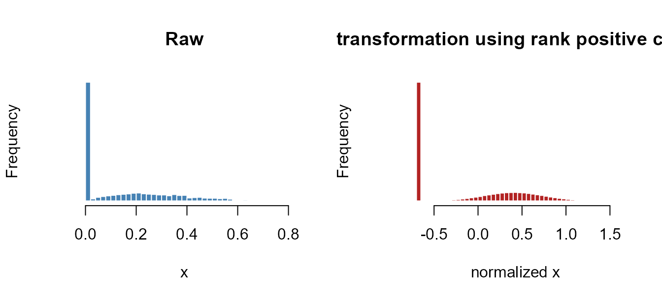
The zero spike is preserved as its own group while the positive component is spread out.
rank_normal — irregular or mixed shapes
Pathology. Anything the parametric transforms can’t
handle gracefully: bimodal distributions, mixed positive/negative
support with no clean model, or a [0, 1] variable piled up
at zero or one. Transform. A rank-based inverse normal
transform maps the empirical mid-ranks onto a Gaussian. Tied values (a
block of exact zeros, say) share the score at the middle of their block,
and because the reference distribution keeps the winsorized tail
observations, clipped values are scored at their actual quantile rather
than at the most extreme normal score. It preserves ordering
but not distances, so it is robust to almost any shape — at the cost of
discarding the original spacing.
set.seed(3)
x_rank <- c(rnorm(1000, -3), rnorm(1000, 4))   # bimodal, mixed support

fit <- find_best_normalization(x_rank, range = "np", verbose = FALSE)
c(type = fit$transform_type,
  raw_kurt = round(fit$raw_kurtosis, 2), fit_kurt = round(fit$fit_kurtosis, 2))
#>          type      raw_kurt      fit_kurt
#> "rank_normal"       "-1.75"       "-0.16"

plot_normalize_x(x_rank, range = "np")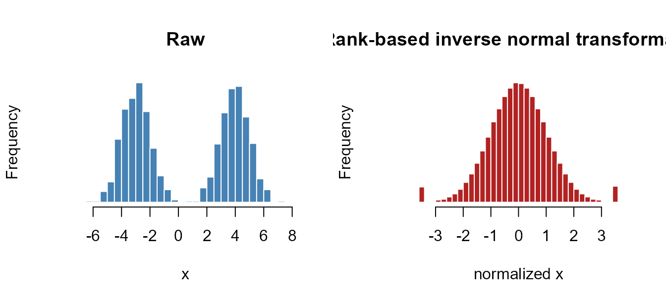
The bimodal shape (strongly negative kurtosis) is pulled toward a single normal mode.
One-step and reusable normalization
normalize_x() runs fit-and-apply in a single call —
handy for a one-off variable:
z <- normalize_x(x_asinh, range = "zp", verbose = FALSE)
round(c(mean = mean(z), sd = sd(z)), 3)
#>  mean    sd
#> 0.315 1.062
When you need the same transformation applied to new data (a different panel year, a holdout sample), fit once and re-apply, so both are scored on an identical scale:
fit  <- find_best_normalization(x_asinh, range = "zp", verbose = FALSE)
z_new <- apply_normalization(rlnorm(50, 10, 1.3), fit = fit)
Force a specific transformation with vtype if you want
to override the auto-detection:
normalize_x(x, range = "np", vtype = "rank_normal")How this connects to the metrics
The _w / _z / _p columns on
every metric come from the winsorize → normalize → rank path shown at
the top (apply_transformations()). The _z
column uses exactly the machinery in this article:
apply_transformations() fits
find_best_normalization() with the metric’s
range (auto-detecting the transformation, so never
hurdle) and scores the ratio with
apply_normalization(). The same transforms matter when
building the fiscal-health index
(vignette("fiscal-health-index")), where each indicator
should be approximately normal before it enters a correlation or factor
model.