Making Governance Scores

#Needed libraries for functionality 
library(data.table)
library(tidyverse)
library(polycor)
library(psych)


## Libraries for Presentation
library(kableExtra)
library(Matrix)
library(ggcorrplot)

How to make a governance score

Here we outline the procedure employed to generate governance scores through factor analysis. Initially, we identify the relevant segments within the 990 efile data containing governance-related information. We then standardize the data into a set of binary variables and conduct a factor analysis. Finally, we calculate governance scores utilizing the loading and weights we derived from the factor model.

We use the 2018 990 efile data as our training data for this model.

Step 0: Identify relevant 990 questions

We first list all questions in the 990 series that we feel indicate governance practices. The questions here have been organized by Part/Schedule of the 990 they are found in.

Part IV

12a. Whether obtained separate, independent audited financial statements (y/n)

12b. Whether organization included in consolidated, independent audited financial statements (y/n)

28a. Whether the organization a party to a business transaction with a current or former officer, director, trustee, or key employee (y/n)

28b. Whether the organization a party to a business transaction to with a family member of a current or former officer, director, trustee, or key employee (y/n)

28c. Whether the organization a party to a business transaction to with an entity of which a current or former officer, director, trustee, or key employee was an officer, director, trustee, or direct or indirect owner (y/n)

Did the organization receive more than 25,000 in non-cash contributions? If yes, complete schedule M. (y/n)
Did the organization receive contributions of art, historical treasures, or other similar assets or qualified conservation contributions? If yes, complete schedule M. (y/n)

*Note that if any “yes” to 29 or 30, org is required to indicate whether it has a “gift acceptance policy” in Schedule M, item 31 (y/n)

Part VI

1a. Number of Voting Members

1b. Number of independent voting members

1.schedule-O. If there are material differences in voting rights among members of the governing body, or if the governing body delegated broad authority to an executive committee or similar committee, explain on Schedule O.

Family relationship or business relationship (y/n)
Whether used a management company or other person to perform any management duties (y/n)
Whether made any significant changes to governing documents (y/n) 5.Whether any significant diversion of assets (y/n)
Whether have members or stockholders (y/n)

7a. Whether have any persons who had power to elect or appoint members(y/n)

7b. Whether decisions reserved to members other than governing body (y/n)

8a. Whether documented the meetings by the governing body (y/n)

8b.Whether documented the meetings by each committee (y/n)

10a. Whether have local chapters, branches, or affiliates (y/n)

10b. If yes to 10a, whether have a written policies governing the activities for local chapters, branches, or affiliates (y/n)

11a. Whether provided a copy of Form 990 to all members before filing the form (y/n)

12a. Whether have a written conflict of interest policy (y/n)

12b. Whether officers, directors, key employees required to disclose annually interests that could give rise to conflicts? (y/n)

12c. Whether regularly and consistently monitor and enforce compliance with the policy (y/n)

Whether have a written whistleblower policy (y/n)
Whether have a written document retention and destruction policy (y/n)

15a. Whether have a process for determining compensation of the CEO, executive director, or top management officials include a review and approval by independent persons, comparability data, and deliberation decision (y/n)

15b. Whether have a process for determining compensation of other officers or key employees include a review and approval by independent persons, comparability data, and deliberation decision (y/n)

16a. Whether invest in, contribute assets to, or participate in a joint venture or similar arrangement (y/n)

16b. If yes 10 16a, whether have a written policy or procedure to evaluate its participation in joint venture or similar arrangements (y/n)

Whether make Forms 1023 (or 1024), 990, 990-T available for public inspection in any of the following forms: Own website, another’s website, upon request, other

Part XII

Accounting method used to prepare the Form 990 in any of the following forms: cash, accrual, other

2a. Were the financial statements compiled or reviewed by an independent accountant* (y/n)

2b. Were the financial statements audited by an independent accountant* (y/n)

2c. If yes to 2a or 2b, whether have a committee that assumes responsibility for oversight of the audit, review, or compilation of its financial statements and selection of an independent accountant? (y/n)

3a. Was required to undergo an audit or audits (y/n)

3b. If yes, did undergo the required audit or audits (y/n)

Schedule M

31 - “Does the organization have a gift acceptance policy that requires the review of any nonstandard contributions?” - only used if Part IV Line 29 or 30 are checked (y/n)

Step 1: Download the 990 Data

We read in the raw 990 efile data from each Part/Schedule for the years we are interested in using as the “base-line” for a governance index. In our case, we use the 2018 data.

years = 2018

We only pull in the columns pertaining to the questions listed in the previous step. See the NCCS Website for a comprehensive data dictionary.

Part IV

### Part IV 

#initialize data
dat_4 <-  vector(mode = "list", length = length(years))
#get columns I want 
keep_cols_part4 <- c("OBJECTID", "URL", "RETURN_VERSION", "ORG_EIN", 
                     "F9_04_AFS_IND_X", "F9_04_AFS_CONSOL_X",
                     "F9_04_BIZ_TRANSAC_DTK_X", "F9_04_BIZ_TRANSAC_DTK_FAM_X", "F9_04_BIZ_TRANSAC_DTK_ENTITY_X",
                     "F9_04_CONTR_NONCSH_MT_25K_X", 
                     "F9_04_CONTR_ART_HIST_X")

for(i in 1:length(years)){
  link <-  paste0("https://nccs-efile.s3.us-east-1.amazonaws.com/parsed/F9-P04-T00-REQUIRED-SCHEDULES-", years[i], ".csv")
  temp <- fread(link, select = keep_cols_part4) 
  colnames(temp) <- c("OBJECTID", "URL", "RETURN_VERSION", "ORG_EIN",
                     "P4_LINE_12A", "P4_LINE_12B",
                     "P4_LINE_28A", "P4_LINE_28B", "P4_LINE_28C",
                     "P4_LINE_29",
                     "P4_LINE_30")
  dat_4[[i]] <- temp
}

#clean up data
dat_all_4 <- 
  rbindlist(dat_4) %>% 
  mutate( year = as.numeric(substr(RETURN_VERSION, 1, 4)))

Part VI

### Part VI 

#initialize data
dat_6 <-  vector(mode = "list", length = length(years))
#get columns I want 
keep_cols_part6 <- c("OBJECTID", "URL", "RETURN_VERSION", "ORG_EIN", 
                     "F9_06_INFO_SCHED_O_X", 
                     "F9_06_GVRN_NUM_VOTING_MEMB",
                     "F9_06_GVRN_NUM_VOTING_MEMB_IND", 
                     "F9_06_GVRN_DTK_FAMBIZ_RELATION_X", 
                     "F9_06_GVRN_DELEGATE_MGMT_DUTY_X",
                     "F9_06_GVRN_CHANGE_DOC_X", 
                     "F9_06_GVRN_ASSET_DIVERSION_X",
                     "F9_06_GVRN_MEMB_STCKHLDR_X", 
                     "F9_06_GVRN_PERS_ELECT_MEMB_X",
                     "F9_06_GVRN_DECISION_APPROV_X",
                     "F9_06_GVRN_DOC_GVRN_BODY_X",
                     "F9_06_GVRN_DOC_COMMITTEE_X",
                     "F9_06_POLICY_CHPTR_AFFIL_X",
                     "F9_06_POLICY_CHPTR_REFERENCE_X",
                     "F9_06_POLICY_FORM990_GVRN_BODY_X",
                     "F9_06_POLICY_COI_X",
                     "F9_06_POLICY_COI_DISCLOSURE_X",
                     "F9_06_POLICY_COI_MONITOR_X",
                     "F9_06_POLICY_WHSTLBLWR_X",
                     "F9_06_POLICY_DOC_RETENTION_X",
                     "F9_06_POLICY_COMP_PROCESS_CEO_X",
                     "F9_06_POLICY_COMP_PROCESS_OTH_X",
                     "F9_06_POLICY_JV_X",
                     "F9_06_POLICY_JV_PROC_X",
                     "F9_06_DISCLOSURE_AVBL_OTH_X",
                     "F9_06_DISCLOSURE_AVBL_OTH_WEB_X",
                     "F9_06_DISCLOSURE_AVBL_REQUEST_X",
                     "F9_06_DISCLOSURE_AVBL_OWN_WEB_X"
                     )

for(i in 1:length(years)){
  link <-  paste0("https://nccs-efile.s3.us-east-1.amazonaws.com/parsed/F9-P06-T00-GOVERNANCE-", years[i], ".csv")
  temp <- fread(link, select = keep_cols_part6) 
  colnames(temp) <- c("OBJECTID", "URL", "RETURN_VERSION", "ORG_EIN",
                     "P6_SCHEDULE_O", 
                     "P6_LINE_1A",
                     "P6_LINE_1B", 
                     "P6_LINE_2", 
                     "P6_LINE_3",
                     "P6_LINE_4", 
                     "P6_LINE_5",
                     "P6_LINE_6",
                     "P6_LINE_7A",
                     "P6_LINE_7B",
                     "P6_LINE_8A",
                     "P6_LINE_8B",
                     "P6_LINE_10A",
                     "P6_LINE_10B",
                     "P6_LINE_11A",
                     "P6_LINE_12A",
                     "P6_LINE_12B",
                     "P6_LINE_12C",
                     "P6_LINE_13",
                     "P6_LINE_14",
                     "P6_LINE_15A",
                     "P6_LINE_15B",
                     "P6_LINE_16A",
                     "P6_LINE_16B",
                     "P6_LINE_18_other", "P6_LINE_18_other_web", "P6_LINE_18_req", "P6_LINE_18_own_web")
  dat_6[[i]] <- temp
}

#clean up data
dat_all_6 <- 
  rbindlist(dat_6) %>% 
  mutate( year = as.numeric(substr(RETURN_VERSION, 1, 4)))

Part XII

### Part XII

#initialize data
dat_12 <-  vector(mode = "list", length = length(years))
#Keep all columns for part XII


for(i in 1:length(years)){
  link <-  paste0("https://nccs-efile.s3.us-east-1.amazonaws.com/parsed/F9-P12-T00-FINANCIAL-REPORTING-", years[i], ".csv")
  temp <- fread(link) 
  dat_12[[i]] <- temp
}

#clean up data
dat_all_12 <- 
  rbindlist(dat_12) %>% 
  mutate( year = as.numeric(substr(RETURN_VERSION, 1, 4)))

Schedule M

#initialize data
dat_M <-  vector(mode = "list", length = length(years))
#get columns I want 
keep_cols_partM <- c("OBJECTID", "URL", "RETURN_VERSION", "ORG_EIN", 
                     "SM_01_REVIEW_PROCESS_UNUSUAL_X")

for(i in 1:length(years)){
  link <-  paste0("https://nccs-efile.s3.us-east-1.amazonaws.com/parsed/SM-P01-T00-NONCASH-CONTRIBUTIONS-", years[i], ".csv")
  temp <- fread(link, select = keep_cols_partM) 
  colnames(temp) <- c("OBJECTID", "URL", "RETURN_VERSION", "ORG_EIN",
                     "PM_LINE_31")
  dat_M[[i]] <- temp
}



#clean up data
dat_all_M <- 
  rbindlist(dat_M) %>% 
  mutate( year = as.numeric(substr(RETURN_VERSION, 1, 4)))

DEVELOPER NOTE We save this version of data in data-raw/data-train-raw.rda.

save(dat_all_4, dat_all_6, dat_all_12, dat_all_M,
     file = "data-raw/dat-train-raw.rda")

Step 2: Wrangle the 990 Data

We wrangle the 990 data from 0/1, X, t/f, or any other raw coding to a communal “yes/no” response (or other if appropriate) according to the “code book” table the respective subsections presented below.

Part IV

Line	Variable	Levels
Line 12A, 12B, 28A, 28B, 28C, 29, 30	P4_LINE_12A, …, P4_LINE_30	“yes” - the answer to this line is yes “no” - the answer to this line is no

#remove any unwanted years that may have accidentally appeared
dat_all_4 <-
  dat_all_4 %>% 
  filter(year <= max(years))

#standardize yes/no answers
dat_all_4 <- 
  dat_all_4 %>% 
  mutate(across(starts_with("P4"), 
                ~ case_when(
                  . %in% c("true", "1") ~ "yes",
                  . %in% c("false", "0") ~ "no", 
                  TRUE ~ .
                )))

Part VI

Line Number	Variable Name	Levels
Line 1A, 1B	P6_LINE_1A, P6_LINE_1B	integer value
Line 2, 3, 4, 5, 6, 7A, 7B, 8A, 8B, 10A, 10B, 11A, 12A, 12B, 12C, 13, 14, 15A, 15B, 16A, 16B	P6_LINE_2, …. , P6_LINE_16B	“yes” - the answer to this line is yes “no” - the answer to this line is no
Line 18	P6_LINE_18	“own_website” - the own website box on line 18 is checked ” others_website” - the another’s website box on line 18 is checked “request” - the upon request website box on line 18 is checked “other” - the other box on line 18 is checked
Line 1 Schedule O	P6_SCHEDULE_O	“X” - there is a Schedule O attached to this return with notes from Part VI Line 1 NA - there is no Schedule O attached to this return with notes from Part VI Line 1

#remove any unwanted years that may have accidentally appeared
dat_all_6 <-
  dat_all_6 %>% 
  filter(year <= max(years))

#general wrangling
dat_all_6 <- 
  dat_all_6 %>% 
  #standardize yes/no answers
  mutate(across(paste0("P6_LINE_", c(2:6, "7A", "7B", "8A", "8B", "10A", "10B", "11A", "12A", "12B", "12C", 13, 14, "15A", "15B", "16A", "16B")) , 
                ~ case_when(
                  . %in% c("true", "1") ~ "yes",
                  . %in% c("false", "0") ~ "no", 
                  TRUE ~ .
                )) ) %>% 
 # Line 18
  mutate(P6_LINE_18 = case_when(
    P6_LINE_18_own_web == "X" ~ "own_website", 
    P6_LINE_18_other_web == "X" ~ "others_website",
    P6_LINE_18_req == "X" ~ "request",
    P6_LINE_18_other == "X" ~ "other"
  )) %>%
  select(-c(P6_LINE_18_own_web,P6_LINE_18_other_web,P6_LINE_18_req, P6_LINE_18_other ))

Part XII

Line Number	Variable Name	Levels
Line 1	P12_LINE_1	“cash” - cash accounting method “accrual” - accrual accounting method “other” - other accounting method
Line 1	P12_L I N E _1_OTHER_EXPLAIN	If P12_LINE_1 is “other”, then this is what is written for other
Line 2a	P12_LINE_2A	“no” - answer to question 2a is no “separate” - answer to question 2a is yes and the box for “separate basis” is checked “colsol” - answer to question 2a is yes and the box for “consolidated basis” is checked “both” - answer to question 2a is yes and the box for “both consolidated and separate basis” is checked
Line 2b Notes: Something is wrong about this coding. There are many F 9 _ 1 2 _FINSTAT_AUDIT_X == FALSE, But F9_12_FIN S T A T _AUDIT_CONSOL_X, F9_12_ F I N S TAT_AUDIT_SEP_X, or F9_12_ F I N S TAT_AUDIT_BOTH_X is checked	P12_LINE_2B	“no” - answer to question 2a is no “separate” - answer to question 2b is yes and the box for “separate basis” is checked “colsol” - answer to question 2b is yes and the box for “consolidated basis” is checked “both” - answer to question 2b is yes and the box for “both consolidated and separate basis” is checked
Line 2C	P12_LINE_2C	“no” - answer to question 2c is no “yes” - answer to question 2c is no
Line 3A	P12_LINE_3A	“no” - answer to question 3a is no “yes” - answer to question 3a is no
Line 3B	P12_LINE_3B	“no” - answer to question 3b is no “yes” - answer to question 3b is no

#remove any unwanted years that may have accidentally appeared
dat_all_12 <-
  dat_all_12 %>% 
  filter(year <= max(years))

## Clean Up Variables
dat_all_12 <-
  dat_all_12 %>% 
  ## Line 1
  mutate(P12_LINE_1 = case_when(
    !is.na(F9_12_FINSTAT_METHOD_ACC_OTH) ~ "other",
    F9_12_FINSTAT_METHOD_ACC_ACCRU_X == "X" ~ "accrual",
    F9_12_FINSTAT_METHOD_ACC_CASH_X == "X" ~ "cash"
  )) %>% 
  mutate(P12_LINE_1_OTHER_EXPLAIN = 
           ifelse(P12_LINE_1 == "other", 
                  F9_12_FINSTAT_METHOD_ACC_OTH,
                  NA)) %>% 
  ### Line 2a
  mutate(temp_2a = case_when(
    F9_12_FINSTAT_COMPILE_X %in% c("true", "1") ~ "1",
    TRUE ~ "0",
  )) %>% 
  mutate(P12_LINE_2A = case_when(
    temp_2a == "0" ~ "no",
    F9_12_FINSTAT_COMPILE_SEP_X == "X" ~ "separate",
    F9_12_FINSTAT_COMPILE_CONSOL_X == "X" ~ "consol",
    F9_12_FINSTAT_COMPILE_BOTH_X == "X" ~ "both"
  )) %>% 
  ### Line 2b
  mutate(temp_2b = case_when(
    F9_12_FINSTAT_AUDIT_X %in% c("true", "1") ~ "1",
    TRUE ~ "0",
  ))  %>% 
  mutate(P12_LINE_2B = case_when(
    temp_2a == "0" ~ "no",
    F9_12_FINSTAT_AUDIT_SEP_X == "X" ~ "separate",
    F9_12_FINSTAT_AUDIT_CONSOL_X == "X" ~ "consol",
    F9_12_FINSTAT_AUDIT_BOTH_X == "X" ~ "both"
  ))%>%
  ### Line 2c
  mutate(P12_LINE_2C = case_when(
    F9_12_FINSTAT_AUDIT_COMMITTEE_X %in% c("true", "1") ~ "yes",
    TRUE ~ "no",
  ))  %>%  
 ### Line 3a
  mutate(P12_LINE_3A = case_when(
    F9_12_FINSTAT_FED_AUDIT_REQ_X %in% c("true", "1") ~ "yes",
    TRUE ~ "no",
  )) %>%
  ### Line 3b
  mutate(P12_LINE_3B = case_when(
    F9_12_FINSTAT_FED_AUDIT_PERF_X %in% c("true", "1") ~ "yes",
    TRUE ~ "no",
  ))  %>% 
  #only keeping relevant variables
  select(OBJECTID,URL, RETURN_VERSION,ORG_EIN,RETURN_TYPE,TAX_YEAR,
         P12_LINE_1,P12_LINE_1_OTHER_EXPLAIN, 
         P12_LINE_2A, P12_LINE_2B, P12_LINE_2C,
         P12_LINE_3A, P12_LINE_3B) %>%
  ### rename year to be consistent with other data.frames
  rename(year = TAX_YEAR)

Schedule M

Line	Variable	Levels
Line 31	PM_LINE_31	“yes” - the answer to this line is yes “no” - the answer to this line is no

#remove any unwanted years that may have accidentally appeared
dat_all_M <-
  dat_all_M %>% 
  filter(year <= max(years))

#standardize yes/no answers
dat_all_M <- 
  dat_all_M %>% 
  mutate(PM_LINE_31 = case_when(
                  PM_LINE_31 %in% c("true", "1") ~ "yes",
                  PM_LINE_31 %in% c("false", "0") ~ "no", 
                  TRUE ~ NA
                ))

Merge all parts into one data set

We exclude all EZ filers from our analysis, as the majority of them typically lack the complete data required for the item responses under consideration. Complete responses are required for training our factor model.


#merge 
#filter out all EZ's
dat_govern <-
  dat_all_4 %>% 
  merge(dat_all_6, by = c("OBJECTID", "URL", "RETURN_VERSION", "ORG_EIN", "year")) %>% 
  merge(dat_all_12, by = c("OBJECTID", "URL", "RETURN_VERSION", "ORG_EIN", "year")) %>% 
  merge(dat_all_M, by = c("OBJECTID", "URL", "RETURN_VERSION", "ORG_EIN", "year")) %>% 
  filter(RETURN_TYPE != "990EZ")

Step 3: Transform 990 Data into features matrix

The first thing we have to do in order to make a features matrix is assign all of our yes/no values to 1 for what we believe are positive governance practices or 0 for what we believe are negative governance practices. i.e.

1 is positive direction (i.e. good governance practices)
0 is negative direction (i.e. bad governance practices)

Variable Name(s)	Original Coding	Design Matrix Coding
P4_LINE_12A P4_LINE_12B	yes/no yes/no	1 - yes to either 12A or 12B 0 - no to both
P4_Line_28A, B, C	yes/no yes/no yes/no	0 - no to all 1 - yes to any of 28A, 28B, or 28C
P4_Line_29 P4_Line_30 PM_LINE_31	yes/no yes/no yes/no/na	1 - (29 no) or (30 no) or (29 yes and PM 31 yes) or (30 yes and PM 31 yes) 0 - (29 yes and PM 31 no) or (30 yes and PM 31 no)
P6_LINE_1A, P6_LINE_1B	numeric	is P6_LINE_1B / P6_LINE_1A >= 0.5 \| i.e. is the proportion of independent members at least 0.5? \|
P6_LINE_2	yes/no	0/1 (no is good)
P6_LINE_3	yes/no	0/1 (no is good)
P6_LINE_4	yes/no	removed, neither yes or no is not good nor bad
P6_Line_5	yes/no	0/1 (no is good)
P6_Line_6	yes/no	removed. neither is good or bad. only answers to P6_Line_7A/B matter
P6_LINE_7A	yes/no	0/1 (no is good)
P6_Line_7B	yes/no	0/1 (no is good)
P6_LINE_10A P6_LINE_10B	yes/no yes/no/NA	1 - (10A no) or (10A yes + 10B yes) 0 - (10A yes + 10B no)
P6_LINE_12B	yes/no/NA	1 - (12A yes + 12B yes) or (12A no) 0 - (12 A yes + 12B no)
P6_LINE_12C	yes/no/NA	1 - (12A yes + 12C yes) or (12A no) 0 - (12 A yes + 12C no)
P6_LINE_16A P6_LINE_16B	yes/no yes/no/NA	1 - (16A no) or (16A yes + 16B yes) 0 - (16A yes + 16B no)
P6_LINE_18	request/own we bsite/another’s website/other	1 - own website 0 - anything else
All other P6_*	yes/no	1/0
P12_LINE_1	Accrual/cash	1 - Accrual 0 - anything else
P12_LINE_2A	both/c on sol/no/seperate	0 - no 1 - anything else
P12_LINE_2B	both/c on sol/no/seperate	0 - no 1 - anything else
P12_LINE_2C	yes/no/NA	1 -( 2B yes + 2C yes ) or (2A yes + 2C yes) or (2a no ) or (2b no) 0- (2a yes and 2c no) or (2b yes and 2c no)
P12_LINE_3A/ P12_LINE_3B	yes/no yes/no	1 - (3a no) + (3a yes +3b yes) 0 - (3a yes + 3b no)

#For P6_LINE_1B / P6_LINE_1A >= 0.625
indep_members_threshold <- 0.5 #this is ~ the median value for this data set


design_mat <- 
  dat_govern %>% 
  #dont need P6_SCHEDULE_O, P12_LINE_1_OTHER_EXPLAIN, RETURN TYPE
  select(- c(P6_SCHEDULE_O, P12_LINE_1_OTHER_EXPLAIN, RETURN_TYPE, P6_LINE_4)) %>%
  #remove all is.na in all columns except P6_LINE_10B, P6_LINE_12B, P6_LINE_12C, P6_LINE_16B, PM_LINE_31
  filter(if_all(-c(P6_LINE_10B, P6_LINE_12B, P6_LINE_12C, P6_LINE_16B, P6_LINE_18, PM_LINE_31), 
                ~ !is.na(.))) %>%
  #P4 Line 12
  mutate(P4_LINE_12 = ifelse(P4_LINE_12A == "yes" | P4_LINE_12B == "yes", 1, 0)) %>%
  select(-c(P4_LINE_12A, P4_LINE_12B))%>%
  #P4 line 28
  mutate(P4_LINE_28 = ifelse(
    P4_LINE_28A == "yes" | 
      P4_LINE_28B == "yes" |
      P4_LINE_28C == "yes" , 0, 1)) %>%
  select(-c(P4_LINE_28A, P4_LINE_28B, P4_LINE_28C)) %>% 
  #P4 line 29 and 30, Schedule M
  mutate(P4_LINE_29_30 = case_when(
    P4_LINE_29 == "yes" & PM_LINE_31 == "no" ~ 0,
    P4_LINE_30 == "yes" & PM_LINE_31 == "no" ~ 0,
    TRUE ~ 1)) %>% 
  select(-c(P4_LINE_29, P4_LINE_30, PM_LINE_31)) %>% 
  #P6_LINE_1 
  filter(P6_LINE_1A != 0) %>% # remove divide by 0 errors
  filter(P6_LINE_1A > P6_LINE_1B) %>% # only keep cases where we have more members than independent members
  mutate(P6_LINE_1 = ifelse(P6_LINE_1B / P6_LINE_1A >= indep_members_threshold, 1, 0)) %>% 
  select(-c(P6_LINE_1B , P6_LINE_1A )) %>%
  #P6_LINE_2, 3, 5, 7A, 7B all have no as good and yes as bad
  mutate_at(vars("P6_LINE_2", "P6_LINE_3", "P6_LINE_5", "P6_LINE_7A", "P6_LINE_7B") ,
            ~ ifelse(. == "no", 1, 0)) %>%
  #P6_Line_10
  mutate(P6_LINE_10 = case_when(
    P6_LINE_10A == "no"  ~ 1,
    P6_LINE_10A == "yes" & P6_LINE_10B == "yes" ~ 1,
    P6_LINE_10A == "yes" & P6_LINE_10B == "no"  ~ 0
  )) %>% 
  select(-c(P6_LINE_10A, P6_LINE_10B)) %>% 
  #P6_LINE_12B
  mutate(P6_LINE_12B = case_when(
    P6_LINE_12A == "no"  ~ 1,
    P6_LINE_12A == "yes" & P6_LINE_12B == "yes" ~ 1,
    P6_LINE_12A == "yes" & P6_LINE_12B == "no"  ~ 0
  )) %>% 
  #P6_LINE_12C
  mutate(P6_LINE_12C = case_when(
    P6_LINE_12A == "no"  ~ 1,
    P6_LINE_12A == "yes" & P6_LINE_12C == "yes" ~ 1,
    P6_LINE_12A == "yes" & P6_LINE_12C == "no"  ~ 0
  )) %>% 
  #P6_LINE_16
  mutate(P6_LINE_16 = case_when(
    P6_LINE_16A == "no"  ~ 1,
    P6_LINE_16A == "yes" & P6_LINE_16B == "yes" ~ 1,
    P6_LINE_16A == "yes" & P6_LINE_16B == "no"  ~ 0
  )) %>% 
  select(-c(P6_LINE_16A, P6_LINE_16B)) %>% 
  # P6_LINE_18 
  mutate(P6_LINE_18 = case_when(
    P6_LINE_18 == "own_website" ~ 1 , 
    is.na(P6_LINE_18) ~ 0,
    TRUE ~ 0
  )) %>% 
  # All other P6 yes is good, no is bad
  mutate_at(vars( paste0("P6_LINE_", c("8A", "8B", "11A", "12A", 13, 14, "15A", "15B"))),
            ~  ifelse(. == "yes", 1, 0)) %>% 
  # P12_LINE_1 
  mutate(P12_LINE_1 = ifelse(P12_LINE_1 == "accrual", 1, 0)) %>% 
  # P12_Line_2A
  mutate(P12_LINE_2A = ifelse(P12_LINE_2A == "no", 0, 1)) %>% 
  # P12_Line_2B
  mutate(P12_LINE_2B = ifelse(P12_LINE_2B == "no", 0, 1)) %>%
  #P12_Line_2C
  mutate(P12_LINE_2C = case_when(
    P12_LINE_2A == "no" ~ 1,
    P12_LINE_2B == "no" ~ 1,
    P12_LINE_2A == "yes" & P12_LINE_2C == "yes" ~ 1,
    P12_LINE_2B == "yes" & P12_LINE_2C == "yes" ~ 1,
    P12_LINE_2A == "yes" & P12_LINE_2C == "no" ~ 0,
    P12_LINE_2B == "yes" & P12_LINE_2C == "no" ~ 0,
    TRUE ~ 0
  )) %>%
  #P12_Line_3
  mutate(P12_LINE_3 = case_when(
    P12_LINE_3A == "no" ~ 1,
    P12_LINE_3A == "yes" & P12_LINE_3B == "yes" ~ 1,
    P12_LINE_3A == "yes" & P12_LINE_3B == "no" ~ 0,
    TRUE ~ 0
  )) %>% 
  select(-c(P12_LINE_3A, P12_LINE_3B)) 
  

#Remove P6_Line_6
design_mat <- 
  design_mat %>% 
  select(-P6_LINE_6)

# nothing is NA
dim(design_mat)
#> [1] 64139    32
dim(na.omit(design_mat))
#> [1] 64113    32

#store ID's to remove from data set for analysis
design_mat_ID <- design_mat[, 1:5]
design_mat <- design_mat[, -(1:5)]

DEVELOPER NOTE We save this version of the data in data-raw/dat-train-wrangled.rda.

save(design_mat, 
     design_mat_ID,
     file = "data-raw/dat-train-wrangled.rda")

Step 4: Exploring correlation structures

Throughout this section we use the polychoric correlations and not the Pearson correlations. This choice is made because all of our features are binary, and polychoric correlations are tailored for ordinal variables. See here for more details on the use of polychoric correlations in factor analysis.

Basic EDA

We first start with some basic exploratory data analysis to see the general structure of our features.

tab_list <- design_mat %>%
  map( function(x) as.data.frame(table(x) ))

tab_summary <-
  rbindlist(tab_list,
          idcol = TRUE,
          fill = TRUE) %>% 
  as.data.frame() %>% 
  mutate(x = paste0("num", x)) %>%
  pivot_wider(names_from = "x", values_from = "Freq") %>%
  mutate(perc0 = round(num0 / (num0 + num1), 3), 
         perc1 = round(num1 / (num0 + num1), 3))%>% 
  arrange(.id)

tab_summary%>%
  kable() %>% 
  kable_styling()

.id	num0	num1	perc0	perc1
P12_LINE_1	22986	41153	0.358	0.642
P12_LINE_2A	63197	942	0.985	0.015
P12_LINE_2B	63197	942	0.985	0.015
P12_LINE_2C	64139	NA	NA	NA
P12_LINE_3	48	64091	0.001	0.999
P4_LINE_12	33827	30312	0.527	0.473
P4_LINE_28	7042	57097	0.110	0.890
P4_LINE_29_30	3821	60318	0.060	0.940
P6_LINE_1	26981	37158	0.421	0.579
P6_LINE_10	102	64037	0.002	0.998
P6_LINE_11A	20598	43541	0.321	0.679
P6_LINE_12A	24219	39920	0.378	0.622
P6_LINE_12B	2908	61212	0.045	0.955
P6_LINE_12C	4647	59491	0.072	0.928
P6_LINE_13	33593	30546	0.524	0.476
P6_LINE_14	31457	32682	0.490	0.510
P6_LINE_15A	38303	25836	0.597	0.403
P6_LINE_15B	44295	19844	0.691	0.309
P6_LINE_16	301	63832	0.005	0.995
P6_LINE_18	59977	4162	0.935	0.065
P6_LINE_2	13764	50375	0.215	0.785
P6_LINE_3	3820	60319	0.060	0.940
P6_LINE_5	63	64076	0.001	0.999
P6_LINE_7A	17610	46529	0.275	0.725
P6_LINE_7B	12013	52126	0.187	0.813
P6_LINE_8A	7530	56609	0.117	0.883
P6_LINE_8B	14324	49815	0.223	0.777

We can see from this table that there are quite a few features that have either all 0’s, all 1’s, or a very small percentage of 0’s and 1’s. Additionally, there are a few features that are perfectly correlated with other features (e.g. P12_LINE_2B and P12_LINE_2A are perfectly correlated) These features probably will not be helpful in our analysis since they do not contain enough variation to tell us anything useful. Let’s remove the features from our analysis that contain less that 2% in either the 0 or 1 class.

### Remove factors where less than 2% in either class 
### This was as small as we could make it in this data set without the correlation matrix being singular
### Remove P12_Line_2B because it is perfectly correlated with 2A
### Remove P6_Line_12B, P6_Line_12C because it is causing singularity issues with P6_Line_12
perc_threshold <- 0.02

#list of variables to keep
vars_keep <- 
  tab_summary %>% 
  filter(perc0 > perc_threshold & perc1 > perc_threshold) %>% 
  filter(.id != "P12_LINE_2B") %>%
  filter(.id != "P6_LINE_12B") %>%
  filter(.id != "P6_LINE_12C") %>%
  pull(.id) %>% 
  sort()

Next we look at the general correlation structure. We can see from the plot below that we have extreme multicollinearity among some of our features. Let’s explore some of these more to decide which ones we want to keep in our analysis.

# make as factor
design_mat_keep <- sapply(design_mat[, ..vars_keep], as.factor) #note the ..vars_keep. the ".." is deliberalty needed in datatable package updates 

#hecor computes polychoric correlations between ordinal variables. 
corr_mat <- hetcor(design_mat_keep, ML = TRUE) #uses maximum likelihood estimates
#> data contain one or more character variables
#> the values of which are ordered alphabetically
#> Warning in hetcor.data.frame(dframe, ML = ML, std.err = std.err, use = use, :
#> the correlation matrix has been adjusted to make it positive-definite

ggcorrplot(corr_mat$correlations,
           hc.order = TRUE ) +
  ggtitle("Correlation Matrix") +
  labs(subtitle = "Variables with More than 2% is either class")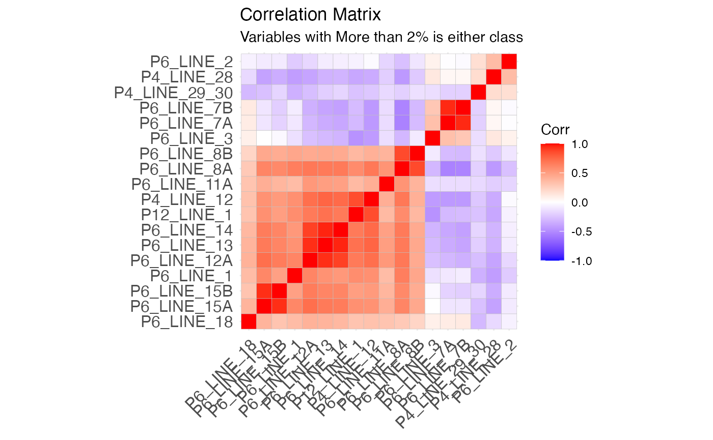

Exploring Highly Correlated Features

Let’s look at which features have a correlation of over 0.90.

dat_cor <- as.data.frame(corr_mat$correlations)
dat_cor$var1 <- rownames(dat_cor) 

dat_cor%>% 
  pivot_longer(!var1, names_to = "var2", values_to = "cor") %>% 
  filter(var1 != var2) %>%
  arrange(desc(abs(cor))) %>%
  filter(abs(cor) >= 0.90)
#> # A tibble: 8 × 3
#>   var1        var2          cor
#>   <chr>       <chr>       <dbl>
#> 1 P6_LINE_13  P6_LINE_14  0.958
#> 2 P6_LINE_14  P6_LINE_13  0.958
#> 3 P6_LINE_7A  P6_LINE_7B  0.949
#> 4 P6_LINE_7B  P6_LINE_7A  0.949
#> 5 P6_LINE_15A P6_LINE_15B 0.939
#> 6 P6_LINE_15B P6_LINE_15A 0.939
#> 7 P6_LINE_12A P6_LINE_13  0.936
#> 8 P6_LINE_13  P6_LINE_12A 0.936

P6_LINE_12A, 13, 14

First, look at correlations of P6_line 12A, 13, 14. They are quite strong so let’s make a new variable, P6_Line_12_13_14, where it is 1 if (P6_Line_13 ==a yes AND P6_Line_14 == yes AND P6_Line_12A == yes) and is 0 otherwise. P6_line 12A, 13, 14 all describe a very similar idea: do you have documented policies?

P6_Line_13 = have whistleblower policy?
P6_Line_14 = have document retention and destruction policy?
P6_Line_12A = Whether obtained separate, independent audited financial statements (y/n)

## All 3 are very correlated
design_mat %>% 
  select(P6_LINE_13, P6_LINE_14, P6_LINE_12A) %>%
  mutate_all(as.factor) %>%
  hetcor(ML = TRUE)
#> 
#> Maximum-Likelihood Estimates
#> 
#> Correlations/Type of Correlation:
#>             P6_LINE_13 P6_LINE_14 P6_LINE_12A
#> P6_LINE_13           1 Polychoric  Polychoric
#> P6_LINE_14      0.9579          1  Polychoric
#> P6_LINE_12A     0.9362     0.8932           1
#> 
#> Standard Errors:
#>             P6_LINE_13 P6_LINE_14
#> P6_LINE_13                       
#> P6_LINE_14    0.001039           
#> P6_LINE_12A   0.001544   0.002071
#> 
#> n = 64139

## Even combing 13 and 14 is still very correlated
design_mat %>% 
  select(P6_LINE_13, P6_LINE_14, P6_LINE_12A) %>%
  mutate(P6_LINE_13_14 = P6_LINE_13 == 1 & P6_LINE_14 == 1) %>%
  select(-c(P6_LINE_13, P6_LINE_14)) %>%
  mutate_all(as.factor) %>%
  hetcor(ML = TRUE)
#> 
#> Maximum-Likelihood Estimates
#> 
#> Correlations/Type of Correlation:
#>               P6_LINE_12A P6_LINE_13_14
#> P6_LINE_12A             1    Polychoric
#> P6_LINE_13_14      0.9305             1
#> 
#> Standard Errors:
#> [1] ""        "0.00171"
#> 
#> n = 64139

design_mat <- 
  design_mat %>% 
  mutate(P6_LINE_12_13_14 = as.numeric(
    P6_LINE_12A == 1 & P6_LINE_13 == 1 & P6_LINE_14 == 1)) %>%
  select(-c(P6_LINE_12A, P6_LINE_13, P6_LINE_14))

Even combining only 2 of the features still leads to high multicollinearity. With this, we conclude that P6_LINE_12A, 13, and 14 should be combined into one feature called P6_Line_12_13_14.

P6_LINE_7A, 7B

P6_7A, 7B are both about having members or stockholders. Let’s make a new variable called P6_Line_7 that is 1 if (P6_Line_7A == yes OR P6_Line_7B == no ) and 0 otherwise. We will also removed Line 6. We think this is reasonable as it may not matter IF you have stock holders, but rather if you do, can they make decisions on behalf of the organization.

P6_LINE_6 = Did the organization have members or stockholders?
P6_Line_7A = Did the organization have members, stockholders, or other persons who had the power to elect one or more members of the governing body?
P6_Line_7B = Are any governance decisions of the organization reserved to (or subject to approval by) members, stockholders, or persons other than the governing body?

design_mat %>% 
  select(P6_LINE_7A, P6_LINE_7B) %>%
  mutate_all(as.factor) %>%
  hetcor(ML = TRUE)
#> 
#> Maximum-Likelihood Estimates
#> 
#> Correlations/Type of Correlation:
#>            P6_LINE_7A P6_LINE_7B
#> P6_LINE_7A          1 Polychoric
#> P6_LINE_7B     0.9456          1
#> 
#> Standard Errors:
#> [1] ""         "0.001531"
#> 
#> n = 64139

design_mat <-
  design_mat %>% 
  mutate(P6_LINE_7 = as.numeric(P6_LINE_7A == 1 & P6_LINE_7B == 1)) %>% 
  select(!c(P6_LINE_7B, P6_LINE_7A))

Ultimately, we choose to remove P6_Line_7 all together because we did not feel addressing questions regarding stakeholders was helpful in the type of governance we wanted to measure. Mathematically, P6_LINE_7 can be included in the factor analysis as it is not highly correlated with any of the other factors, but we excluded for reasons pertaining to interpretation.

P6_LINE_15A, 15B

We choose to keep P6_Line_15A as it describes the main idea that we care about in these line items. Additionally, through observation we know that most organizations are not doing one or the other; most do both or neither.

P6_LINE_15A = compensation review and approval for CEO?
P6_LINE_15B = compensation review and approval for other officers and key employees?

design_mat %>% 
  select(P6_LINE_15A, P6_LINE_15B) %>%
  mutate(P6_LINE_15A = as.factor(P6_LINE_15A),
         P6_LINE_15B = as.factor(P6_LINE_15B)) %>% 
  hetcor(ML = TRUE)
#> 
#> Maximum-Likelihood Estimates
#> 
#> Correlations/Type of Correlation:
#>             P6_LINE_15A P6_LINE_15B
#> P6_LINE_15A           1  Polychoric
#> P6_LINE_15B      0.9388           1
#> 
#> Standard Errors:
#> [1] ""        "0.00146"
#> 
#> n = 64139

design_mat <-
  design_mat %>% 
  select(-P6_LINE_15B)

P6_LINE_8B

We may also want to remove P6_Line_8B. It is causing non-positive-definite issues and is very highly correlated with 8A. Similar to above, both items tell a similar sentiment.

8a.Whether documented the meetings by the governing body (y/n)
8b.Whether documented the meetings by each committee (y/n)

design_mat %>% 
  select(P6_LINE_8A, P6_LINE_8B) %>%
  mutate(P6_LINE_8A = as.factor(P6_LINE_8A),
         P6_LINE_8B = as.factor(P6_LINE_8B)) %>% 
  hetcor(ML = TRUE)
#> 
#> Maximum-Likelihood Estimates
#> 
#> Correlations/Type of Correlation:
#>            P6_LINE_8A P6_LINE_8B
#> P6_LINE_8A          1 Polychoric
#> P6_LINE_8B     0.9656          1
#> 
#> Standard Errors:
#> [1] ""         "0.001519"
#> 
#> n = 64139

design_mat <-
  design_mat %>% 
  select(-P6_LINE_8B)

Looking at the correlations again

Let’s look at our new correlation structure.

#### Trying the Correlations Again without the problematic variables

#updated the variables to keep
#add the variables I added
adding <- c("P6_LINE_12_13_14")
vars_keep2 <- c(vars_keep, adding) 
 #remove the variables I removed
removing <- c("P6_LINE_7A", "P6_LINE_7B",
              "P6_LINE_13", "P6_LINE_14", "P6_LINE_12", "P6_LINE_12A",
              "P6_LINE_15B", 
              "P6_LINE_8B",
              "P6_LINE_7")

vars_keep2 <- vars_keep2[!(vars_keep2 %in% removing)]

design_mat2 <- sapply(design_mat[, ..vars_keep2], as.factor) #note the ..vars_keep. the ".." is deliberalty needed in datatable package updates 


corr_mat2 <- hetcor(design_mat2, ML = TRUE)
#> data contain one or more character variables
#> the values of which are ordered alphabetically

ggcorrplot(corr_mat2$correlations,
           hc.order = TRUE ) +
  ggtitle("Correlation Matrix") +
  labs(subtitle = "Variables with More than 3% is either class")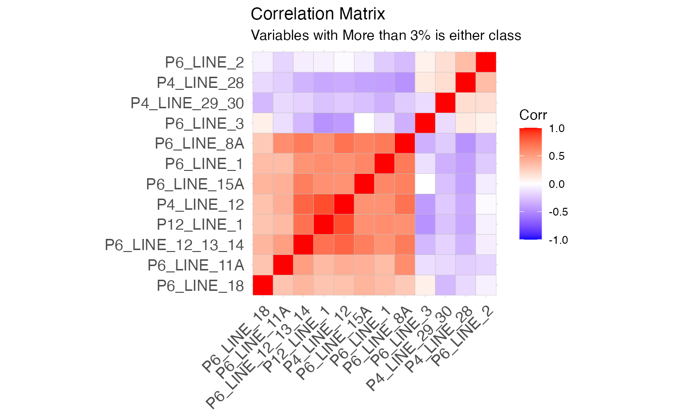

This looks like a much more reasonable correlation structure to work with!

DEVELOPER NOTE We save this version of the data as (data-raw/dat-train-final.rda)[https://github.com/Nonprofit-Open-Data-Collective/governance/blob/main/data-raw/dat-train-final.rda].

save(design_mat2, 
     design_mat_ID,
     file = "data-raw/dat-train-final.rda")

Step 5: Pick final fetures to go into factor analysis

We choose to use P12_LINE_1, P4_LINE_12, P4_LINE_28, P4_Line_29_30, P6_Line_1, P6_Line_2, P6_Line_3, P6_Line_8A, P6_Line_11A, P6_Line_12_13_14, P6_Line_15A, and P6_Line_18 as our factors for the analysis.

Summary of Variables Used in Index

All variables are coded as 1 (good governance practice) or 0 (bad governance practice)

Feature Name ========= P4_ LINE _12A	Feature Meaning/Coding \| \| \| ==============================================+ Did the org obtain separate, independent \| audited financial statements? 1 - yes, 0 - \| no \|
Feature Name ========= P4_ LINE _12A
P4 _LIN E_28	1- Answered “no” to questions P4_LINE_28A, P4_LINE_28B, AND P4_LINE_28 0 - Answered yes to any of these questions Essentially 1 if no business was done with a family member and 0 otherwise.
P 4_LI NE_2 9_30	1- (Answered no to P4_LINE_29 ANDP4_Line_30) \| or (Answered yes to (P4_LINE_29 \| OR P4_Line_30) AND answered yes to Schedule \| M question 31 ) \| 0 - Answered yes to (P4_LINE_29 \| OR P4_Line_30) AND answered no to Schedule \| M Line 31 \| \| i.e. 1 if either (the org did not have more \| than $25K in cash contribution AND did not \| have receive any art/historical \| treasures/etc.) OR (they do have those \| things AND they do have a written policy \| about how to handle them) \|
P 6_LI NE_1	1 - The proportion of independent members on the board is at least 50% 0 - The proportion of independent members on the board is less than 50%
P 6_LI NE_2	1- No officer, director, trustee, or key employee had a family relationship or a business relationship with any other officer, director, trustee, or key employee 0- An officer, director, trustee, or key employee had a family relationship or a business relationship with any other officer, director, trustee, or key employee
P 6_LI NE_3	1- The org did not use a management company or other person to perform any management duties 0 - The org did use a management company or other person to perform any management duties
P6 _LIN E_8A	1 - The meetings by the governing body are documented 0 - The meetings by the governing body are not documented
P6_L INE_ 12_1 3_14	1- The answers to P6_Line_12, 13, and 14 are all yes 0- otherwise i.e. 1 if the organization has a written conflict of interest policy, AND a written whistleblower policy, AND a written retention and destruction policy. These 3 are combined because seperated they have >0.90 correlation. And all of these questions get at the same type of governance - do you have written policies for when things go bad?
P6_ LINE _11A	1- A copy of Form 990 is provided to all members before filing the form 0 - otherwise
P6_ LINE _15A	1- The org has a process for determining compensation of the CEO, executive director, or top management officials including a review and approval by independent persons, comparability data, and deliberation decision 0 - otherwise
P6 _LIN E_18	1 - Forms 1023 (or 1024), 990, 990-T available for public inspection on own website 0 - These forms were listed on another’s website, available upon request, or “other”
P1 2_LI NE_1	Did the org use accrual method for accounting? 1 - yes, 0- no

Summary of Features Not Used in Index

Feature Name	Reason why it is not used
P4_LINE_12B	Perfectly correlated with P4_Line_12A
P6_LINE_4	Removed, neither good nor bad
P6_Line_5	Less than 2% in 0 category
P6_Line_6	Removed, neither good nor bad
P6_LINE_7A, P6_LINE_7B	Causing singularity issues
P6_Line_8B	Perfectly correlated with P6_Line_8A
P6_Line_12B, P6_LINE_12C	Folded into question 12A,
P6_LINE_15A	Perfectly correlated with P6_Line_15A
P6_LINE_16A, P6_LINE_16B	Less than 2% in 0 category
P12_LINE_2A, P12_LINE_2C	Less than 2% in 1 category
P12_LINE_2B	Perfectly correlated with P12_Line_2A

#make the features matrix
features2 <-  matrix( 
  as.numeric(design_mat2), ncol = ncol(design_mat2)) 

colnames(features2) <- colnames(design_mat2)

## Polychoric correlation
poly_cor2 = psych::polychoric(features2)
rho2 = poly_cor2$rho

Step 6: Run the Factor Analysis

We choose to use the “equamax” rotation in our factor analysis. We want independent factors, and equamax balances simplifying the factors (from varimax) and simplifying the variables (quartimax). See here for details on rotation types.

Pick the number of factors

Before we can run a factor analysis, we use the scree plot to pick the number of factors we want to consider.

We choose to use 6 factors based on the plot below and after testing the interpretability of our results.

fa.parallel(rho2, 
            fm="mle", 
            fa="fa", 
            main = "Scree Plot",
            cor = "poly",
            nfactors = 1,
            n.obs = nrow(design_mat_keep))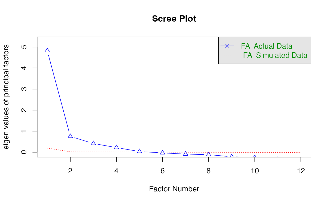

#> Parallel analysis suggests that the number of factors =  5  and the number of components =  NA

Run the factor analysis:

Once we have decided we will use 6 factors, we run the factor analysis model.

set.seed(98435)
model6 = fa(features2, nfactor=6, cor="poly", fm="mle", rotate = "equamax")
#> Loading required namespace: GPArotation
model6$loadings
#> 
#> Loadings:
#>                  ML1    ML2    ML4    ML3    ML6    ML5   
#> P12_LINE_1        0.654  0.103  0.422  0.372  0.221  0.274
#> P4_LINE_12        0.825  0.346  0.244  0.259  0.241       
#> P4_LINE_28       -0.170 -0.294 -0.244               -0.425
#> P4_LINE_29_30    -0.204        -0.117  0.214 -0.164 -0.413
#> P6_LINE_1         0.280  0.401  0.424         0.167  0.421
#> P6_LINE_11A       0.111  0.362  0.130         0.605       
#> P6_LINE_15A       0.248  0.346  0.729         0.260  0.150
#> P6_LINE_18        0.203         0.243 -0.150  0.397  0.185
#> P6_LINE_2         0.163 -0.226                      -0.509
#> P6_LINE_3        -0.181 -0.115        -0.920              
#> P6_LINE_8A        0.246  0.816  0.281  0.213  0.296  0.236
#> P6_LINE_12_13_14  0.466  0.289  0.445  0.204  0.439       
#> 
#>                  ML1   ML2   ML4   ML3   ML6   ML5
#> SS loadings    1.711 1.446 1.379 1.230 1.043 0.998
#> Proportion Var 0.143 0.121 0.115 0.102 0.087 0.083
#> Cumulative Var 0.143 0.263 0.378 0.480 0.567 0.651
fa.diagram(model6)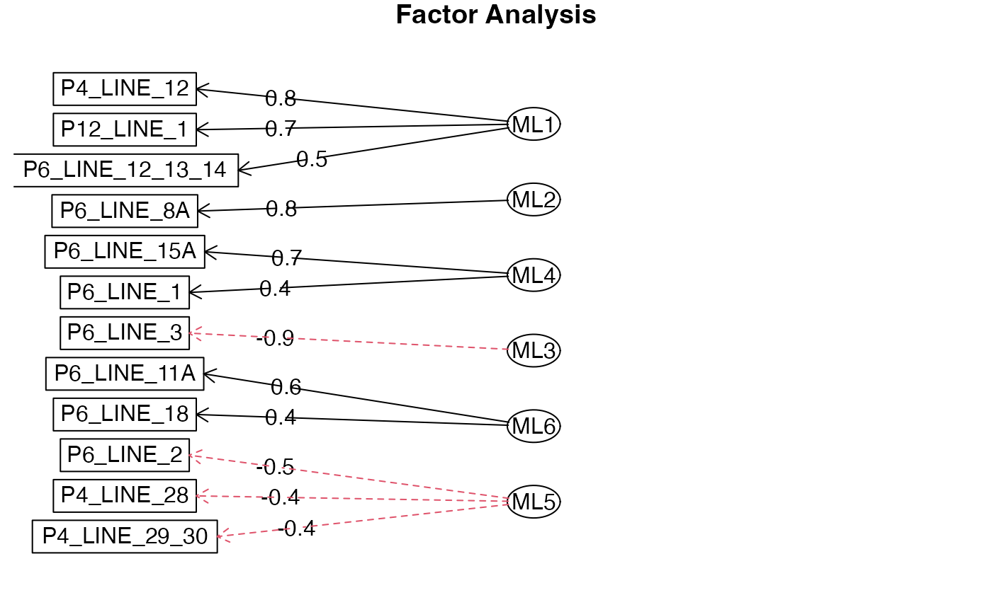

Cumulatively, we explain ~65% of the variance in our data set, which is a value we are comfortable with.

Adding Factor Scores

The original fa function from the psych package will calculate factor scores, but since our factors are binary, the fa$scores output are not the factor scores we are interested in. The fa function defaults to using Pearson correlations in the score calculation even if it uses polychoric correlations in the factor loadings calculation.

Instead, we use the factor.scores function to specify the exact method we wish to use when calculating our factor scores.

We need to specify the exact correlation (polychoric) structure we are using to calculate our factor scores.
We need to specify “Thurstone” method to use the “regression based weights” when calculating the scores.
For each organization, we first find the score loaded onto each factor, then use the sum of those 6 factor scores as the total score.

scores <- factor.scores(features2, #data to caluculate scores on 
                        model6,  #model object 
                        rho = polychoric(features2)$rho, #polychoric correlation
                        method = "Thurstone") #method of calculating scores


all.dat <- cbind(features2, scores$scores)
all.dat <- as.data.frame(all.dat)

all.dat$total.score <- rowSums(scores$scores)
hist(all.dat$total.score,
     main = "Histogram of Total Scores in Original Data",
     xlab = "total score")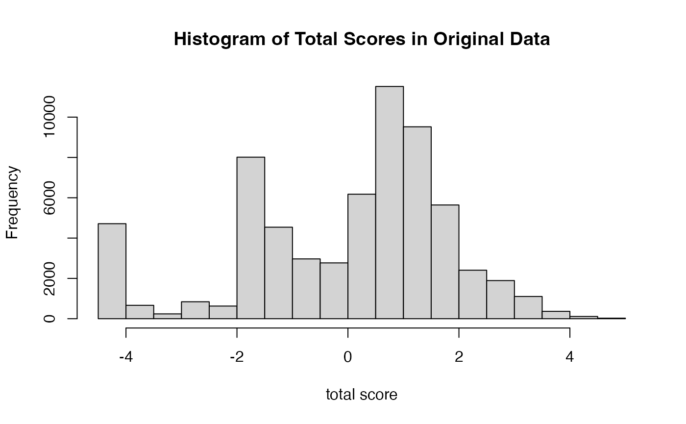

DEVELOPER NOTE We save the features matrix and factor analysis object in data/factor-objects.rda.

dat.2018 <- cbind(design_mat_ID, all.dat)
save(dat.2018,
     features2,
     scores,
     model6,
     rho2,
     file = "data/factor-objects.rda")

Step 7: Interpret the Factors

Variables( positive meaning i.e. value = 1)	Factor Group Names
P12_Line_1: Accounting method is accural (bad is anything else) P4_Line_12: The organization obtains separate, independent audited financial statements P6_Line_12_13_14: The organization has a written conflict of interest policy, a written whistleblower policy, and a written retention and destruction policy	Have doc umentable/ written accounting practices and general policies
P6_LINE_8A: The meetings by the governing body are documented Correlated with 8b. meetings by each committee are documented	Open d ocumenting of orga nizational business
P6_LINE_15A: The org has a process for determining compensation of the CEO, executive director, or top management officials including a review and approval by independent persons, comparability data, and deliberation decision Correlated with Line 15b. The org has a process for determining compensation of other officers or key employees includin a review and approval by independent persons, comparability data, and deliberation decision P6_Line_1: The percent of independent members on the voting board is >50%	Good policies for making the board and for paying them
(Negative) P6_LINE_3: The org did not use a management company or other person to perform any management duties	The or ?did? using a management company
P6_Line_11A: A copy of Form 990 is provided to all members before filing the form P6_Line_18: Forms 1023 (or 1024), 990, 990-T available for public inspection on own website	IRS forms are available for public inspection
(Negative) P4_Line_28: The org was not a party to a business transaction to with an entity of which a current or former officer, director, trustee, or key employee was an officer, director, trustee, or direct or indirect owner (Negative) P6_Line_2: No officer, director, trustee, or key employee had a family relationship or a business relationship with any other officer, director, trustee, or key employee? (Negative) P4_Line_29: Either (the org did not have more than $25K in cash contribution AND did not have receive any art/historical treasures/etc.) OR (they do have those things AND they do have a written policy about how to handle them)	These are all about doing business with family or having large/ expensive assets

Step 8: Calculate scores for new data

We demonstrate how factor scores can be caluculated for a new data set.

First, we generate new data.

#make new data that "somewhat" resembles the original data
N <- 100
new.data <- matrix(NA, ncol = ncol(features2), nrow = N)
colnames(new.data) <- colnames(features2)
for(i in 1:ncol(features2)){
  new.data[, i] <- rbinom(N, 1, mean(features2[, i]))
}

Then we calculate new scores using the factor.scores function from the psych package. Note the options we use are exactly the same as calculating scores for the original data, we just now use our new data. It is important to use the correlation structure of the original data, rho2, when doing this correlation, otherwise, the results will not be interpretable.

new.scores<- factor.scores(new.data,  #new data 
                        model6, #model object 
                        rho = rho2, #polychoric corrlations of original data
                        method = "Thurstone") #method of calculating scores

Appendix:

A1: Calculating Factor Scores

In this Appendix, we show the “by-hand” calculations for how we do the “Thurstone” method of calculating factor scores given the factor loadings.

There are 12 features, 6 factors, and n $\approx$ 64k observations. Let,

$D$ = the Design matrix $\in \mathbb{R}^{n x 12}$
$D_S$ = Design matrix with columns centered at 0 and scaled to have 1 sd $\in \mathbb{R}^{n x 12}$
$C$ = observed correlation matrix $\in \mathbb{R}^{12 x 12}$ . In our example, this is the polychoric correlation.
$L$ = factor loading matrix $\in \mathbb{R}^{12 x 6}$ . This is calculated from the fa function.
$W = C^{-1}L$ = matrix of weights ($\beta$ ’s in the regression model) $\in \mathbb{R}^{12 x 6}$
$S = D_s W$ = matrix of scores $\in \mathbb{R}^{n x 6}$

Thus if $D_s^*$ is a new (scaled) design matrix using the same scaling mean and sd as $D_S$ , then $S^* = D_s^* W$$ is the matrix of new scores. (The factor.scores function automatically scales the $D$ matrix in its calculation).

# from above: 
# scores <- factor.scores(features2, 
#                         model6, 
#                         rho = polychoric(features2)$rho,
#                         method = "Thurstone")

data.scaled <- scale(features2)
D <- data.scaled
C <- model6$r  # =  polychoric(features2)$rho
W <- scores$weights
L <- model6$loadings #same as model6$Structure
S <- scores$scores
n <- nrow(features2)

#S = DW so lets check ||DW - S|| ~=0
sum(abs((D %*% W) - S))
#> [1] 0

#W = C^(-1) L so lets check  ||C^(-1) L - W|| ~=0
sum(abs(solve(C) %*% L - W))
#> [1] 1.552541e-14

If we were to get new data, this is how we would get the new scores. It is important to use the correlation matrix of the original data set so that the score results are interpretable.

scaled.mean <- attr(data.scaled, "scaled:center")
scaled.sd <- attr(data.scaled, "scaled:scale")

N <- 100
new.data <- matrix(NA, ncol = ncol(features2), nrow = N)
colnames(new.data) <- colnames(features2)
for(i in 1:ncol(features2)){
  new.data[, i] <- rbinom(N, 1, mean(features2[, i]))
}

new.scores<- factor.scores(new.data, 
                        model6, 
                        rho = polychoric(features2)$rho,
                        method = "Thurstone")

Note about how `psych` package calculates scores

Scores should be calculated as $DC^{-1}L$, where $L$ was calculated from the fa function using the polychoric correlations. Thus, we want the scores to be $S = DC^{-1}_{polychoric}L$. However, even when you specify for the fa function to use polychoric correlations when calculating $L$, they will always use Pearson correlations when calculating the scores. Thus the scores object in the fa output will always be $S_{default} = DC^{-1}_{Pearson}L$. Since we are interested in the polychoric correlations, we need to calculate the scores using the factor.scores function to have more control over which correlation matrix is used.

## Default scores 
S.defult <- model6$scores

## Pearson Corelation
C.pearson <- cor(features2)

## Polychoric Correlation
C.poly <- rho2

## What we want 
S.poly <- D %*% solve(C.poly) %*% L
# show that ||S.polychoric - factor.scores output|| ~= 0
sum(abs(scores$scores - S.poly)) #approx 0
#> [1] 3.243303e-10

## What the `fa` funciton gives us
S.pearson <- D %*% solve(C.pearson) %*% L
# show that ||S.default - fa output|| ~=0 
sum(abs(S.defult - S.pearson)) #approx 0
#> [1] 5.567155e-08

#But S.poly =/= S.pearson
sum(abs(S.defult - S.poly))
#> [1] 161480.4

Olivia Beck

2024-03-14

How to make a governance score

Step 0: Identify relevant 990 questions

Part IV

Part VI

Part XII

Schedule M

Step 1: Download the 990 Data

Part IV

Part VI

Part XII

Schedule M

Step 2: Wrangle the 990 Data

Part IV

Part VI

Part XII

Schedule M

Merge all parts into one data set

Step 3: Transform 990 Data into features matrix

Step 4: Exploring correlation structures

Basic EDA

Exploring Highly Correlated Features

P6_LINE_12A, 13, 14

P6_LINE_7A, 7B

P6_LINE_15A, 15B

P6_LINE_8B

Looking at the correlations again

Step 5: Pick final fetures to go into factor analysis

Summary of Variables Used in Index

Summary of Features Not Used in Index

Step 6: Run the Factor Analysis

Pick the number of factors

Run the factor analysis:

Adding Factor Scores

Step 7: Interpret the Factors

Step 8: Calculate scores for new data

Appendix:

A1: Calculating Factor Scores

Note about how psych package calculates scores

Note about how `psych` package calculates scores