Governance Workflow

library(governance)
library(dplyr)
library(ggplot2)

This vignette walks through the full path from raw 990 fields to governance scores and shows a few ways to explore the results.

Step 1: Get input data

get_features() consumes raw 990 efile fields from Part IV, Part VI, Part XII, and Schedule M. In production these come from the companion panel990 package via get_governance_data(years = 2022); see vignette("download-data") for the field list, the required tables, and the full-990 filter. Here we use the bundled example, a 5,000-organization sample of raw 2022 fields.

data("dat_example", package = "governance")

set.seed(57)
dat_example <- dat_example[sample(seq_len(nrow(dat_example)), 200), ]

Step 2: Build the feature matrix

get_features() cleans the raw fields and appends 12 binary governance features. Blank or missing yes/no responses are treated as 0 regardless of how the source encoded them (NA or ""), so results do not depend on how the tables were read.

features_example <- get_features(dat_example)

features_example |>
  select(ORG_EIN, starts_with("P6_"), P12_LINE_1) |>
  head()
#>        ORG_EIN P6_LINE_1 P6_LINE_11A P6_LINE_12_13_14 P6_LINE_15A P6_LINE_18
#> 849  521314461         1           1                1           1          0
#> 2532 832563658         1           0                0           0          1
#> 2699 870470748         0           1                1           1          0
#> 2478 752538361         1           1                0           0          0
#> 531  650144766         1           0                0           0          0
#> 3673 883636365         0           0                0           0          0
#>      P6_LINE_2 P6_LINE_3 P6_LINE_8A P12_LINE_1
#> 849          1         1          1          1
#> 2532         1         1          1          1
#> 2699         1         1          1          1
#> 2478         0         1          1          0
#> 531          0         1          1          1
#> 3673         1         1          0          0

Each feature is an indicator of a good-governance practice. We can look at how common each practice is in the sample:

feature_cols <- c("P12_LINE_1", "P4_LINE_12", "P4_LINE_28", "P4_LINE_29_30",
                  "P6_LINE_1", "P6_LINE_11A", "P6_LINE_15A", "P6_LINE_18",
                  "P6_LINE_2", "P6_LINE_3", "P6_LINE_8A", "P6_LINE_12_13_14")

rates <- features_example |>
  summarise(across(all_of(feature_cols), ~ mean(.x == 1, na.rm = TRUE))) |>
  tidyr::pivot_longer(everything(), names_to = "feature", values_to = "rate")

ggplot(rates, aes(x = reorder(feature, rate), y = rate)) +
  geom_col() +
  coord_flip() +
  labs(title = "Share of organizations passing each governance feature",
       x = NULL, y = "Share == 1")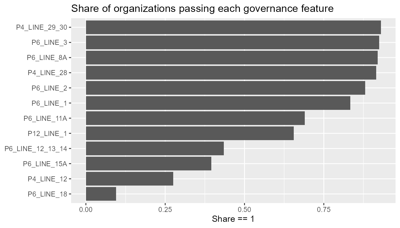

Step 3: Calculate the scores

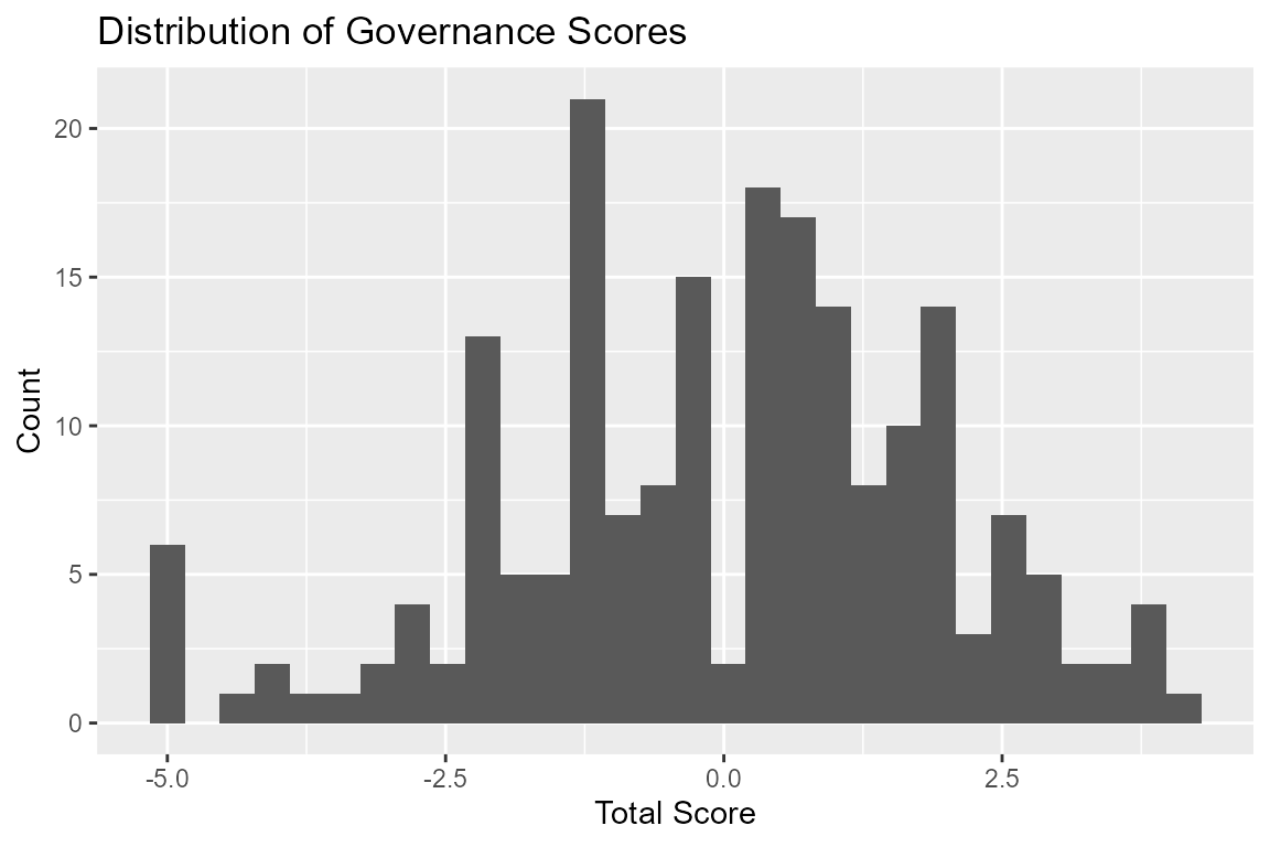
get_scores() applies the pre-fit factor model and appends six factor scores and a total.score.

scores_example <- get_scores(features_example)

scores_example |>
  select(ORG_EIN, total.score) |>
  head()
#>        ORG_EIN total.score
#> 849  521314461  1.84480679
#> 2532 832563658  1.41783202
#> 2699 870470748 -0.08681385
#> 2478 752538361 -0.27424699
#> 531  650144766  0.60652413
#> 3673 883636365 -5.00061728

ggplot(scores_example, aes(x = total.score)) +
  geom_histogram(bins = 30) +
  labs(
    title = "Distribution of Governance Scores",
    x = "Total Score", y = "Count"
  )

Joining external data (optional)

Governance scores are most useful alongside other organizational characteristics. You can join the scores to the NCCS Business Master File (BMF) on ORG_EIN to relate governance to size, sector, or geography. The snippet below is illustrative (not run here, as it downloads a large file):

library(readr)
library(stringr)

# Unified BMF (single file across years)
bmf_url <- paste0(
  "https://nccsdata.s3.us-east-1.amazonaws.com/",
  "bmf/unified/v1.2/UNIFIED_BMF_V1.2.csv"
)
bmf <- read_csv(bmf_url)
bmf$EIN <- str_pad(gsub("\\D", "", bmf$EIN), 9, pad = "0")

plot_data <- scores_example |>
  left_join(bmf, by = c("ORG_EIN" = "EIN"))

ggplot(plot_data, aes(x = log(ASSETS), y = total.score)) +
  geom_point(alpha = 0.4) +
  labs(title = "Governance Scores vs. Total Assets",
       x = "log(Total Assets)", y = "Total Governance Score")

Governance Workflow

Olivia Beck

2026-08-11